Introduction

Gradient descent is a popular method applied almost everywhere in machine learning. But back to the period that traditional mathematics rules the world, ordinary least square is the fundamental of solving linear problem. Therefore, my motivation of writing this blog is to figure out the similarity and difference of these two methods.

Hopefully after this, we will have better understanding on the aspect of both theory and experiments.

Theory

While I was reviewing Machine Learninxg by Andrew Ng, the course skipped the proof part of OLS, by default thinking that we have sufficient matrix knowledge (do we? lol). So, I’d like to include the proof here.

First, let’s introduce some terminologies and notations. Consider a multiple linear regression:

\[h_{\boldsymbol \theta}(\boldsymbol x^{(i)}) = \theta_0 + \theta_1 x_1^{(i)} + \theta_2 x_2^{(i)} + … + \theta_n x_n^{(i)} = \boldsymbol \theta^T \boldsymbol x^{(i)} = {\boldsymbol x^{(i)}}^T \boldsymbol \theta \] where $\boldsymbol \theta = \begin{bmatrix} \theta_0 \\ \theta_1 \\ \vdots \\ \theta_n \end{bmatrix}$， $\boldsymbol x^{(i)} = \begin{bmatrix} 1 \\ x_1^{(i)} \\ x_2^{(i)} \\ \vdots \\ x_n^{(i)} \end{bmatrix}$， $\boldsymbol y = \begin{bmatrix} y_1 \\ y_2 \\ \vdots \\ y_m \end{bmatrix}$

$\boldsymbol y$ is the target，$h_{\boldsymbol \theta}(\boldsymbol x^{(i)})$ is the hypothesis function, $m$ is number of training samples / observations, $n$ is number of features, e.g. $\boldsymbol x^{(i)}$ is the $ith$ training sample, $x_j^{(i)}$ is the $jth$ feature value of ith training sample.

Given the cost function: \[J(\boldsymbol \theta) = \frac{1}{2m} \sum_{i=1}^m (h_{\boldsymbol \theta}(\boldsymbol x^{(i)}) - y_i)^2\]

The objective is to estimate parameters $\boldsymbol \theta$, so that hypothesis function can have the minimum cost.

Gradient Descent

Since the cost function is a convex bowl-shaped graph, let’s use a 2-dimension projection between $J$ and $\theta_i$ to explain how the algorithm works.

2-dimension projection looks like:

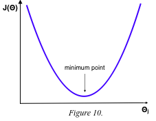
In order to get the minimum point, the algorithm will start from a higher point $\theta_i$, using learning rate and derivatives / slope through many iterations until it gets there. Both derivaties $\frac{\partial J}{\partial \boldsymbol \theta}$ and learning rate $\alpha$ will impact on how fast the algorithm goes until it reaches the bottom. If $\alpha$ is too large, it can bring in divergent problem too. Because of this, normalization and wisely choose $\alpha$ within the model becomes important.

Now the expression of gradient descent becomes: $ {\theta}_j := {\theta}_j - \alpha \frac {\partial J(\boldsymbol \theta)} {\partial \theta_j} $

Furthermore we have:

$\frac {\partial J(\boldsymbol \theta)} {\partial \theta_j} = \frac{1}{m} \sum_{i=1}^m (h_{\boldsymbol \theta}(\boldsymbol x^{(i)}) - y_i) \ \frac {\partial h_{\boldsymbol \theta}(\boldsymbol x^{(i)})} {\partial \theta_j} = \frac{1}{m} \sum_{i=1}^m (h_{\boldsymbol \theta}(\boldsymbol x^{(i)}) - y_i) \ \frac {\boldsymbol x^{(i)} \partial {\boldsymbol \theta}^T} {\partial \theta_j} = \frac{1}{m} \sum_{i=1}^m (h_{\boldsymbol \theta}(\boldsymbol x^{(i)}) - y_i) \ \boldsymbol x^{(i)}$,

This satisfies all except $\theta_0$, which the derivatives part is equal to 1 as $\theta_0$ is a constant.

Finally, the algorithm becomes (repeat until convergence):

$${\theta}_0 := {\theta}_0 - \alpha \frac{1}{m} \sum_{i=1}^m (h_{\boldsymbol \theta}(\boldsymbol x^{(i)}) - y_i)$$ $$\vdots$$ $${\theta}_n := {\theta}_n - \alpha \frac{1}{m} \sum_{i=1}^m (h_{\boldsymbol \theta}(\boldsymbol x^{(i)}) - y_i) \ \boldsymbol x^{(i)}$$

Note that parameters $\theta_0$, $\theta_1$, …, $\theta_n$ must be updated simultaneously in gradient descent.

Ordinary Least Square

Have $\sum_{i=1}^m (h_{\boldsymbol \theta}(\boldsymbol x^{(i)}) - y_i)^2 = \begin{bmatrix} h_{\boldsymbol \theta}(\boldsymbol x^{(1)}) - y_1 \ \dots\ h_{\boldsymbol \theta}(\boldsymbol x^{(m)}) - y_m \end{bmatrix} \times \begin{bmatrix} h_{\boldsymbol \theta}(\boldsymbol x^{(1)}) - y_1 \\ \vdots\\ h_{\boldsymbol \theta}(\boldsymbol x^{(m)}) - y_m \end{bmatrix}$ $= \begin{bmatrix} \boldsymbol \theta^T \boldsymbol x^{(1)} - y_1 \ \dots\ \boldsymbol \theta^T \boldsymbol x^{(m)} - y_m \end{bmatrix} \times \begin{bmatrix} \boldsymbol \theta^T \boldsymbol x^{(1)} - y_1 \\ \vdots\\ \boldsymbol \theta^T \boldsymbol x^{(m)} - y_m \end{bmatrix}$

Also have $\begin{bmatrix} \boldsymbol \theta^T \boldsymbol x^{(1)} - y_1 \\ \vdots\\ \boldsymbol \theta^T \boldsymbol x^{(m)} - y_m \end{bmatrix} =\begin{bmatrix} \boldsymbol \theta^T \boldsymbol x^{(1)} \\ \vdots\\ \boldsymbol \theta^T \boldsymbol x^{(m)} \end{bmatrix} - \boldsymbol y =\begin{bmatrix} {\boldsymbol x^{(1)}}^T \boldsymbol \theta \\ \vdots\\ {\boldsymbol x^{(m)}}^T \boldsymbol \theta \end{bmatrix} - \boldsymbol y = \boldsymbol X \boldsymbol \theta - \boldsymbol y$,

where $\boldsymbol X = \begin{bmatrix} {\boldsymbol x^{(1)}}^T \\ \vdots\\ {\boldsymbol x^{(m)}}^T \end{bmatrix} = \begin{bmatrix} 1 & x_1^{(1)} & x_2^{(1)} & \dots & x_n^{(1)}\\ \vdots\\ 1 & x_1^{(m)} & x_2^{(m)} & \dots & x_n^{(m)}\end{bmatrix}_{m \times (n+1)}$

Therefore have:

$$\sum_{i=1}^m (h_{\boldsymbol \theta}(\boldsymbol x^{(i)}) - y_i)^2 = (\boldsymbol X \boldsymbol \theta - \boldsymbol y)^T (\boldsymbol X \boldsymbol \theta - \boldsymbol y)$$

Regardless $\frac{1}{2m}$, the cost function then can be simplified as:

$$J(\boldsymbol \theta) = (\boldsymbol X \boldsymbol \theta - \boldsymbol y)^T (\boldsymbol X \boldsymbol \theta - \boldsymbol y)$$ $$J(\boldsymbol \theta) = ((\boldsymbol X \boldsymbol \theta)^T - {\boldsymbol y}^T) (\boldsymbol X \boldsymbol \theta - \boldsymbol y) = {\boldsymbol \theta}^T {\boldsymbol X}^T \boldsymbol X \boldsymbol \theta - (\boldsymbol X \boldsymbol \theta)^T \boldsymbol y - {\boldsymbol y}^T \boldsymbol X \boldsymbol \theta + {\boldsymbol y}^T \boldsymbol y$$

Note that $(\boldsymbol X \boldsymbol \theta)^T \boldsymbol y= {\boldsymbol y}^T \boldsymbol X \boldsymbol \theta$, because both $\boldsymbol X \boldsymbol \theta$ and $\boldsymbol y$ are vectors and have the same dimensions, so the order to multiply does not matter.

Then:

$$J(\boldsymbol \theta) = {\boldsymbol \theta}^T {\boldsymbol X}^T \boldsymbol X \boldsymbol \theta - 2 (\boldsymbol X \boldsymbol \theta)^T \boldsymbol y + {\boldsymbol y}^T \boldsymbol y$$

Therefore to get the minimum cost, calculate derivatives:

$$\frac{\partial J}{\partial \boldsymbol \theta} = \frac {\partial ({\boldsymbol \theta}^T {\boldsymbol X}^T \boldsymbol X \boldsymbol \theta - 2 (\boldsymbol X \boldsymbol \theta)^T \boldsymbol y + {\boldsymbol y}^T \boldsymbol y)}{\partial \boldsymbol \theta} = \frac {\partial ({\boldsymbol \theta}^T {\boldsymbol X}^T \boldsymbol X \boldsymbol \theta)}{\partial \boldsymbol \theta} - \frac {\partial (2 (\boldsymbol X \boldsymbol \theta)^T \boldsymbol y)}{\partial \boldsymbol \theta} = \frac {({\boldsymbol X}^T \boldsymbol X) \partial ({\boldsymbol \theta}^T \boldsymbol \theta)}{\partial \boldsymbol \theta} - \frac {2 (\boldsymbol X \boldsymbol y) \partial {\boldsymbol \theta}^T }{\partial \boldsymbol \theta} = 0$$

where $ \boldsymbol X$ and $\boldsymbol y$ are constants.

Furthermore, recall matrix calculus can infer that: $\partial {\boldsymbol \theta}^T \boldsymbol \theta = 2 \boldsymbol \theta, \partial {\boldsymbol \theta}^T = {(\partial \boldsymbol \theta)}^T = 1$

Therefore we have:

$$\frac{\partial J}{\partial \boldsymbol \theta} = 2 {\boldsymbol X}^T \boldsymbol X \boldsymbol \theta - 2 {\boldsymbol X}^T \boldsymbol y \boldsymbol= 0$$

Finally, obtain the normal equation as:

$$\boldsymbol \theta = ({\boldsymbol X}^T {\boldsymbol X})^{-1} {\boldsymbol X}^T \boldsymbol y$$

Experiments

Since these two methods solve the same problem from different perspectives, first question would be will they end up having the same estimation result?

Short answer to this – Yes, and it should not be a surprise…

Here’s an article that took the experiment with a linear regression generated by small size of random points: OLS vs Gradient Descent Experiment.

According to the article, the estimate of intercept $\theta_0$ is 6.089, and the estimate of slope $\theta_1$ is 0.767 based on OLS. And here below is the overview of GD:

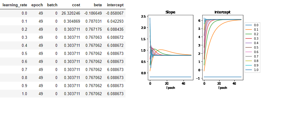
In addition, the article compared simulation result of mini-batch GD vs OLS, which comes up with the conclusion that min-batch GD will not be convergent due to having non-shuffled data during training and inappropriate learning rate.

Similarity and difference

Under most situation, you can choose to use either ordinary least square or gradient descent. With small dataset or relatively small number of features (~<$10^4$), OLS is preferred. However, if features # is too large, should consider using gradient descent as it would compute faster.

Here below lists the difference between OLS and GD:

• GD requires to choose $\alpha$ and do iteration, but OLS doesn’t
• OLS requires to compute $({\boldsymbol X}^T {\boldsymbol X})^{-1}$, which have rare cases that matrix is non-invertible, so you may have to reduce dimensions or avoid multicollinearity
• OLS is slower than GD when features # is large

In the end, it also exists normal equation in nonlinear least square, which I suppose can be another discussion compared with gradient descent later.